Preparing the data for the automated dashboard article

(Note 2026-09-02: This is a technical archive from 2019. The interfaces, links, files and practices involving Universal Analytics, Google Analytics and Kaggle are described as they existed when the article was published.)

Data sources

For the online store, I used 2017 data from the Google Merchandise Store, which I manually exported to CSV files. A better method would be to use one of the many packages that provide access to the Analytics Reporting API. The Google Analytics demo account did not allow API access, however, so I exported all the required files by hand.

For the physical store, I created a sample file by heavily modifying data from a UK retailer. The original data is available on Kaggle.

I also created a Kaggle page containing the final files used on this page.

Starting the project

We first need the following packages:

tidyverse, a collection of packages containing everything we need to prepare the data.
readr, a faster and more intuitive package for reading CSV files.

# Load packages
library(tidyverse)

library(readr)

The first step is to import the data. Here I use a local file, but it is also possible to make HTTP requests for a file on a server or GET requests to an API with the httr package. By default, read_csv does not convert columns containing letters to numeric columns because doing so could discard data. We therefore need to ask it explicitly to remove dollar and percentage signs.

# Import data
Online_original <- read_csv("All_Transactions_SKU.csv", 
    skip = 6)

KEY_TransactionID_Date <- read_csv("KEY_TransactionID_Date.csv")

KEY_SKU_ProductName <- read_csv("KEY_SKU_ProductName_GOOGLE.csv", 
    skip = 6)

KEY_SKU_Category <- read_csv("KEY_SKU_Category_Google.csv", 
    skip = 6)

# Convert columns containing $ or % signs
Online_original$"Product Revenue" <- parse_number(Online_original$"Product Revenue")
Online_original$"Avg. Price" <- parse_number(Online_original$"Avg. Price")

KEY_SKU_Category$"Product Revenue" <- parse_number(KEY_SKU_Category$"Product Revenue")
KEY_SKU_Category$"Avg. Price" <- parse_number(KEY_SKU_Category$"Avg. Price")
KEY_SKU_Category$"Product Refund Amount" <- parse_number(KEY_SKU_Category$"Product Refund Amount")
KEY_SKU_Category$"Basket-to-Detail Rate" <- parse_number(KEY_SKU_Category$"Basket-to-Detail Rate")
KEY_SKU_Category$"Buy-to-Detail Rate" <- parse_number(KEY_SKU_Category$"Buy-to-Detail Rate")

KEY_SKU_ProductName$"Product Revenue" <- parse_number(KEY_SKU_ProductName$"Product Revenue")
KEY_SKU_ProductName$"Avg. Price" <- parse_number(KEY_SKU_ProductName$"Avg. Price")
KEY_SKU_ProductName$"Product Refund Amount" <- parse_number(KEY_SKU_ProductName$"Product Refund Amount")
KEY_SKU_ProductName$"Basket-to-Detail Rate" <- parse_number(KEY_SKU_ProductName$"Basket-to-Detail Rate")
KEY_SKU_ProductName$"Buy-to-Detail Rate" <- parse_number(KEY_SKU_ProductName$"Buy-to-Detail Rate")

KEY_TransactionID_Date$"Revenue" <- parse_number(KEY_TransactionID_Date$"Revenue")
KEY_TransactionID_Date$"Tax" <- parse_number(KEY_TransactionID_Date$"Tax")
KEY_TransactionID_Date$"Delivery" <- parse_number(KEY_TransactionID_Date$"Delivery")
KEY_TransactionID_Date$"Refund Amount" <- parse_number(KEY_TransactionID_Date$"Refund Amount")

Next, we filter the imported files so we retain only one type of category, unique transaction IDs for dates and unique product SKUs for product information. We then join all the tables into a single table containing all the information and remove what is not relevant.

# Filter the category table to retain only one category type
KEY_SKU_Category <- filter(KEY_SKU_Category, 
                          `Product Category (Enhanced E-commerce)` == "Accessories"|
                          `Product Category (Enhanced E-commerce)` == "Android"|
                          `Product Category (Enhanced E-commerce)` == "Apparel"|
                          `Product Category (Enhanced E-commerce)` == "Backpacks"|
                          `Product Category (Enhanced E-commerce)` == "Bags"|
                          `Product Category (Enhanced E-commerce)` == "Bottles"|
                          `Product Category (Enhanced E-commerce)` == "Drinkware"|
                          `Product Category (Enhanced E-commerce)` == "Fun"|
                          `Product Category (Enhanced E-commerce)` == "Gift Cards"|
                          `Product Category (Enhanced E-commerce)` == "Google"|
                          `Product Category (Enhanced E-commerce)` == "Headgear"|
                          `Product Category (Enhanced E-commerce)` == "Housewares"|
                          `Product Category (Enhanced E-commerce)` == "Lifestyle"|
                          `Product Category (Enhanced E-commerce)` == "More Bags"|
                          `Product Category (Enhanced E-commerce)` == "Nest"|
                          `Product Category (Enhanced E-commerce)` == "Nest-Canada"|
                          `Product Category (Enhanced E-commerce)` == "Nest-USA"|
                          `Product Category (Enhanced E-commerce)` == "Notebooks & Journals"|
                          `Product Category (Enhanced E-commerce)` == "Office"|
                          `Product Category (Enhanced E-commerce)` == "Waze"
                          )

# Remove duplicates from KEY_TransactionID_Date (transaction IDs 45426 and 33673, probably manual corrections to erroneous orders)
KEY_TransactionID_Date <- distinct(KEY_TransactionID_Date, `Transaction ID`, .keep_all = TRUE)

# Remove duplicates from KEY_SKU_ProductName
KEY_SKU_ProductName <- distinct(KEY_SKU_ProductName, `Product SKU`, .keep_all = TRUE)

# Remove duplicates from KEY_SKU_Category
KEY_SKU_Category <- distinct(KEY_SKU_Category, `Product SKU`, .keep_all = TRUE)

# Join the data from all tables
Online_joined <- left_join(Online_original, KEY_TransactionID_Date, by = "Transaction ID")
Online_joined <- left_join(Online_joined, KEY_SKU_ProductName, by = "Product SKU")
Online_joined <- left_join(Online_joined, KEY_SKU_Category, by = "Product SKU")

# Retain only relevant columns and reorder them
Online <- select(Online_joined, "Transaction ID", "Date", "Product SKU", "Product", "Product Category (Enhanced E-commerce)", "Quantity.x", "Avg. Price.x", "Revenue", "Tax", "Delivery" )

# Rename columns carrying duplicate indicators now that they are no longer needed
colnames(Online)[colnames(Online)=="Quantity.x"] <- "Quantity"
colnames(Online)[colnames(Online)=="Avg. Price.x"] <- "Avg. Price"

Our sample file of online-store transactions is ready!

Creating the physical-store file

Because I am publishing the data used in this example, I cannot use the private data on which I normally perform this kind of work. I therefore decided to use a file from Kaggle and adapt it to the present situation.

First, we read the original “UK Retailer” file from Kaggle: https://www.kaggle.com/carrie1/ecommerce-data

# Read the original file
Retail_original <- read_csv("UK retailer data.csv")

# Remove returns
Retail_clean <- Retail_original %>% filter(Quantity > 0)

We now modify the purchase dates so they cover only January 1 through December 31, 2017, as in our ecommerce file.

# Load lubridate, which makes dates easier to work with
library(lubridate)

# Convert the character column to a date and remove the time information
Retail_clean$InvoiceDate <- as.Date(Retail_clean$InvoiceDate, format = "%m/%d/%Y")

# Add one month and six years, then subtract one day from every date
Retail_clean$InvoiceDate <- Retail_clean$InvoiceDate %m+% months(1)
Retail_clean$InvoiceDate <- Retail_clean$InvoiceDate %m+% years(6)
Retail_clean$InvoiceDate <- Retail_clean$InvoiceDate %m-% days(1)

# Remove anything outside 2017
Retail_clean <- Retail_clean %>% filter(InvoiceDate < "2018-01-01" & InvoiceDate > "2016-12-31")

We now simulate the purchased quantities and store them until we apply them to our file.

# Visualize online-store quantities after removing outliers
freqs <- Online %>% group_by(Quantity) %>% tally()

# Remove outliers
freqs <- freqs %>% filter(Quantity <= 10)

# Visualize
ggplot(data = freqs, aes(x = Quantity, y = n)) + 
  geom_point() +
  xlim(0, 10)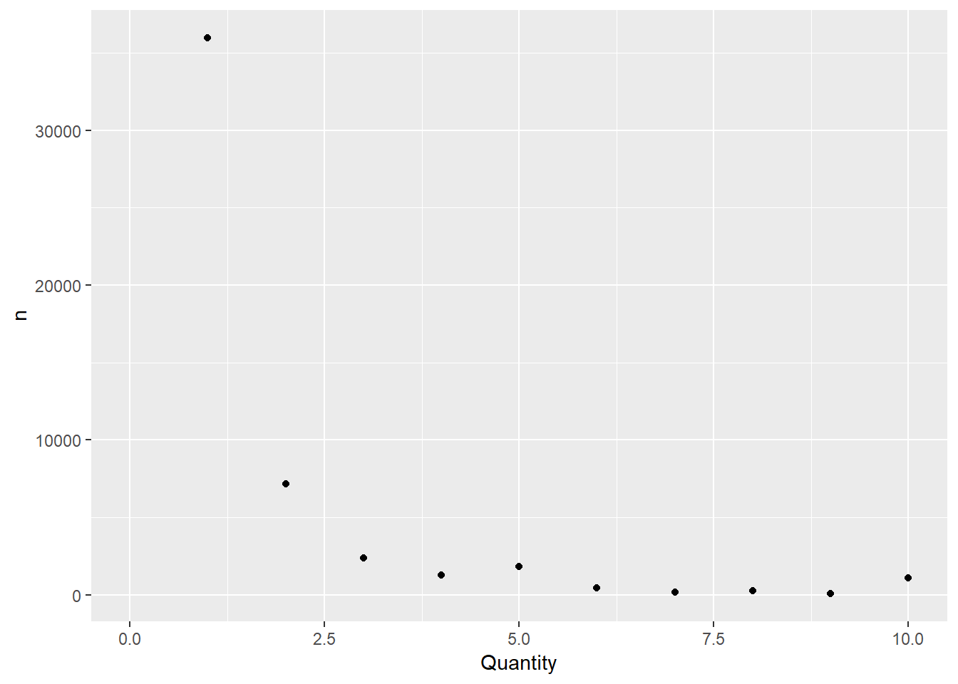

Distribution of quantities purchased from the online store.

(Note 2026-09-02: The physical-store data is fictional. This code does not set a seed, so its results are not deterministic and may vary from one execution to another.)

# Create random quantities using the online store's distribution for our physical-store data

den <- density(Online$Quantity, na.rm = TRUE)

den_qty <- round(sample(Online$Quantity, 505882, replace=TRUE) + rnorm(505882, 0, den$bw), digits = 0)

den_qty <- as.data.frame(den_qty)

# Replace NAs created by rounding with 1...
den_qty <- den_qty %>% mutate(den_qty = if_else(is.na(den_qty), 1, den_qty))

# Check whether the distribution looks similar to the original...
freqs2 <- den_qty %>% group_by(den_qty) %>% tally()

# Remove outliers
freqs2 <- freqs2 %>% filter(den_qty <= 10)

ggplot(data = freqs2, aes(x = den_qty, y = n)) + 
  geom_point() +
  xlim(0, 10)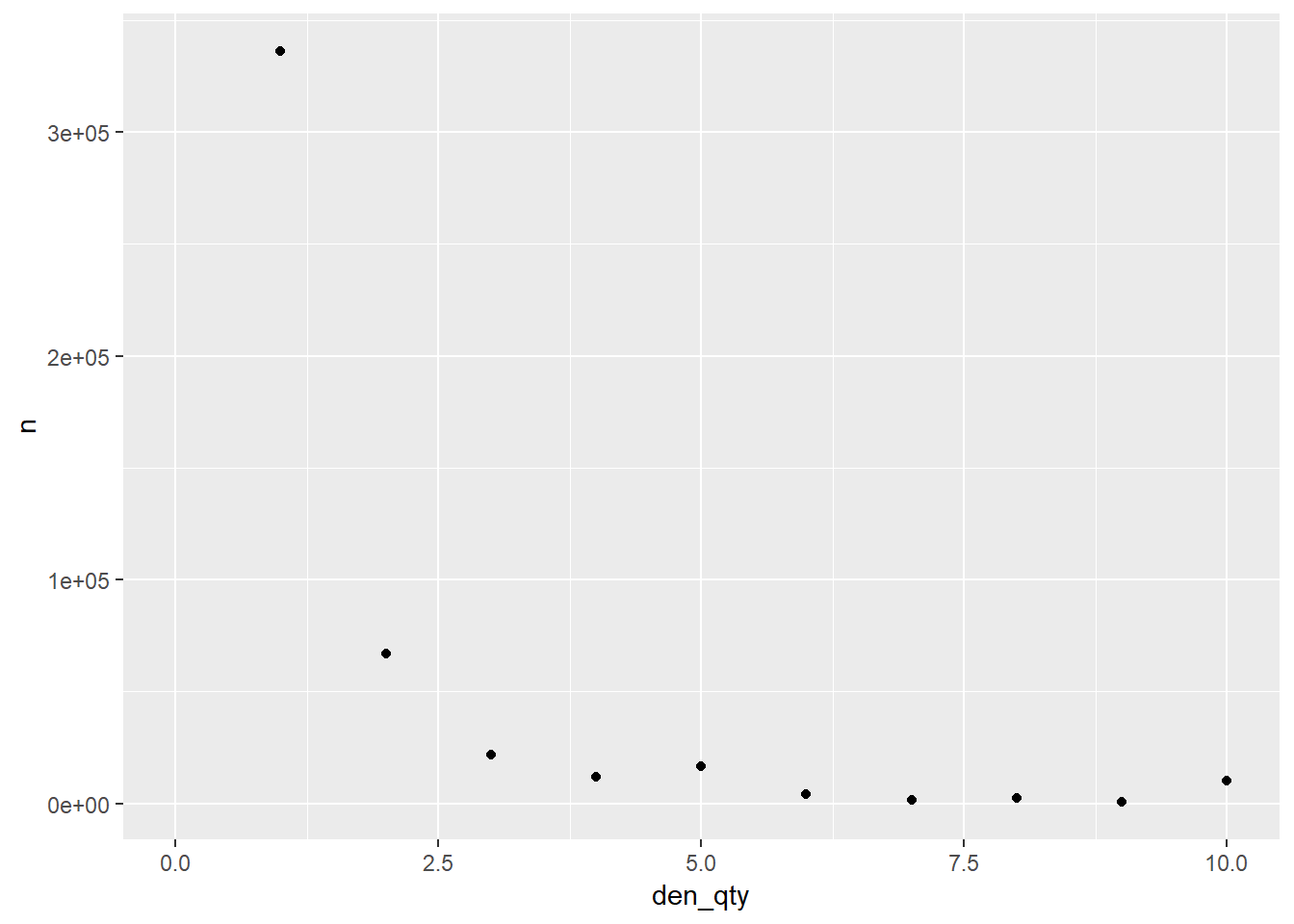

Simulated distribution of quantities purchased for the physical-store data.

# It does!

We now join the data for our fictional file, retaining only the date, stock code and invoice number columns and using our previous data for purchased quantities. We are simulating a file with very little information, which we will enrich in the example.

# Create the file
Retail <- data.frame(InvoiceNo = Retail_clean$InvoiceNo, InvoiceDate = Retail_clean$InvoiceDate, StockCode = Retail_clean$StockCode, Quantity = den_qty$den_qty, stringsAsFactors = FALSE)

Finally, we reduce the number of SKUs in the Retail file until it equals the number in the Online file. This will allow us to create a key between the two files in the next example.

# Count SKUs in the Online file
nrow(as.data.frame(unique(Online$`Product SKU`)))

## [1] 1178

# 1,178 unique SKUs.

# Count SKUs in the Retail file
nrow(as.data.frame(unique(Retail$StockCode)))

## [1] 3931

# 3,931 unique SKUs. That is too many!

# Reduce the number of SKUs in the Retail file by nearly three quarters without reducing the number of transactions too much. Start by cleaning SKUs that use a letter for variations so we retain only numeric SKUs.

Retail$StockCode <- str_replace(Retail$StockCode, "[a-zA-Z]\b$", "")

# How many SKUs do we have now?
nrow(as.data.frame(unique(Retail$StockCode)))

## [1] 3309

# 3,309 SKUs. Still too many.

# Remove SKUs that represent errors (BANKCHARGES, POS, etc.), along with the entire transaction.

Retail <- Retail %>% filter(str_detect(StockCode, "\d\d\d\d\d"))

# We can now convert the column to numeric form because it no longer contains letters

Retail$StockCode <- parse_number(Retail$StockCode)

# How many SKUs do we have now?
nrow(as.data.frame(unique(Retail$StockCode)))

## [1] 3288

# 3,288 SKUs. We will remove orders arbitrarily to reach our goal. Remember, this is only a sample file!

# Create a table of our unique SKUs to identify the first 1,178
unique_retail_SKUS <- as.data.frame(sort(unique(Retail$StockCode)))

# The first 1,178 SKUs range from 10002 to 22314. Exclude every row containing a purchase of a SKU outside this range.

Retail <- Retail %>% filter(StockCode <= 22314)

# How many SKUs do we have now?
nrow(as.data.frame(unique(Retail$StockCode)))

## [1] 1178

# 1,178 SKUs. We have reached our goal!

That’s it! Both files are ready for the example. Visit it here: Automated dashboard example with R and Google Compute Engine

Data sources

Starting the project

Creating the physical-store file

Third time's the charm - Why this site rebuild was completed when others attempts failed